Les Bases de la Fonction de Tranfert

Introduction au Concept de Mesure > Les Bases de la Fonction de Tranfert

A transfer function measurement is a comparison of the a signal going into a system under test to the signal that comes out. By examining the differences between the input signal and the output we can infer the frequency response of the system, both its magnitude and phase response, without really needing to know much about what happened in between – the assumption being that any differences between the signal that went into the system and the signal that came out had to be the result of something that the system did to the original signal. A general term for this strategy is System Identification.

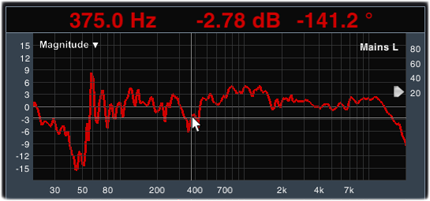
Figure 1: Transfer Function Magnitude display.

On a transfer function Magnitude display, since we are looking at only the differences between the input and the output signals of the system under test, a system with perfectly flat frequency magnitude response would read as a flat line at 0 dB. At frequencies where the magnitude trace is above the zero line it's an indication that the signal came out hotter than that went in, typically due to amplification or acoustic resonance. At frequencies where the magnitude traces below the zero line, the system has attenuated the input signal in some fashion.

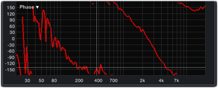
Figure 2: Transfer Function Phase display.

Similarly, the transfer function Phase display tells us how the timing of the input signal was affected as it passed through the system, as a function of frequency. Again, if the system were perfectly transparent in terms of its time response, we would end up with a flat line on the phase display at 0°. If not, we will see some amount of phase shift indicating that some frequencies pass through the system more quickly or slowly than others. Phase shift is plotted in degrees, based on the cycle time for each frequency where 360° (+/–180°) represents the time required for one complete cycle at any given frequency.

Transfer function measurements enable us to evaluate the frequency magnitude and phase response of a system very precisely. They can also be inverse Fourier transformed to find the impulse response of the system, which is an extremely useful tool for finding delay times and evaluating reflections, reverberant decay, and other acoustical properties of the system. The transfer function of a system can be measured using any one of several techniques. the common thread in all of them is that the signal that goes into the system to produce a given output must be precisely known. This is also the thing that most clearly differentiates transfer function measurements from single-channel spectral analysis techniques that directly evaluate only the output of a system.

System identification techniques such as maximal length sequence (MLS) analysis or time delay spectrometry (TDS) are stimulus-dependent, requiring the use of known input signals – i.e., sweeps or pseudorandom noise sequences. MLS and TDS were both popular in early acoustic measurement systems because they required relatively little computing power compared to FFT-based transfer function analyzers. Another approach however is to simply take the discrete Fourier transforms (DFT) of both the input and output signals and divide them (in practice, FFTs are almost always used for the sake of efficiency). This dual-port approach is by far the most flexible of these three techniques because it allows you to directly measure the input signal, rather than needing to know what it is in advance.

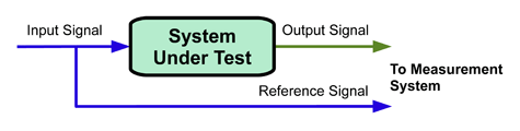
Figure 3: Basic signal routing for a dual-port, FFT-based Transfer Function measurement.

When dual-FFT transfer function measurements are made using pseudorandom noise or sweep sequences that are matched in the length to the the size of the DFTs, they can yield lab quality measurement results with noise rejection characteristics comparable to stimulus dependent measurement systems. But the added capability of dual FFT transfer function analyzers to produce high quality measurement results using random, uncorrelated signals opens up some really interesting additional possibilities. For example you can EQ a system using the type of program material is meant to reproduce and actually hear what you're doing while you're doing it. This also makes it possible to test or monitor the performance of the signal while it's actually in service.

 
Figure 4: Signal routing for a transfer function measurement of a simple sound system.

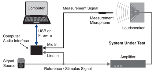
Figure 4 above illustrates basic signal routing for a transfer function measurement of a simple sound system. In this example a music player provides the stimulus signal for the system under test (an amplifier and loudspeaker) as well as the reference signal for the measurement system. The measurement system consists of a computer, a measurement microphone, and a standard USB or FireWire computer audio interface. The measurement microphone picks up the output of the system under test. The audio interface digitizes the two analog signals (reference and measurement) and sends the digital signals to the computer for analysis. In this case we will assume that the audio interface also provides phantom power and pre-amplification for the measurement microphone, meaning no additional preamp is required.