Les Bases de la Réponse Impulsionnelle

Introduction au Concept de Mesure > Les Bases de la Réponse Impulsionnelle

An impulse response is the time domain response of a system under test to an impulsive stimulus. You can actually measure the impulse response of the system by sending pulse through it in some fashion. This is sometimes referred to as an "imperfect" impulse response measurement owing to the difficulty of creating a perfectly instantaneous impulse.

To directly measure the impulse response of acoustics systems, i.e. rooms, people have resorted to such things as popping balloons, gunshots, signal cannon, burning bits of wire with a spot welder, or or simply whacking two boards or other hard objects together and recording the results. In fact all these tactics are still fairly commonly used to measure the impulse response of acoustic spaces where no sound system is present.

When a sound system is present however, a more attractive option may be to measure the transfer function of the system using a continuous test signal such as pink noise, then calculate the impulse response of the system by simply taking the inverse Fourier transform (IFT) of the transfer function. This approach will give you more consistently repeatable results that are actually much closer to what the systems response to an ideally impulsive stimulus would be that any of the methods mentioned above.

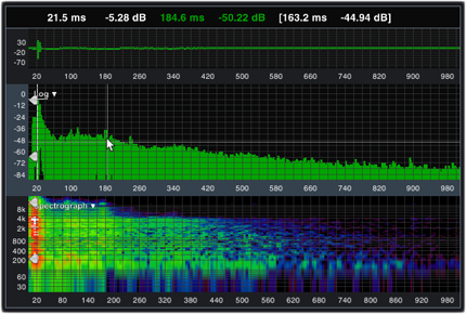
A time domain impulse response plot (above) with a spectrograph below.

In Smaart we use impulse response measurements calculated from the system transfer function to find delay times for real-time transfer function measurements in the frequency domain. In Impulse Response mode you can also measure much larger impulse responses suitable for room acoustics analysis and analyze them in both the time and frequency domains. Impulse Response (IR)Mode is accessed by clicking the Impulse button immediately below the Signal Level/SPL Meter in Real Time mode, or by selecting IR Mode from the Mode menu.

IR Mode features an impulse response recorder that can measure the impulse response of the system using FFT sizes up to 512k points, yielding FFT time constants of up to 11.9 seconds at 44.1k sampling rate. This is sufficient to measure the impulse response of rooms the size of domed stadiums without dropping the sampling rate and sacrificing high-frequency content for the sake of the longer time constant. Since smarts impulse response recorder works by measuring the transfer function of the system under test and then taking its inverse Fourier transform, measurement set up in signal routing for impulse response measurements is identical to configuring the measurement system for a transfer function measurement. See the topics on Transfer Function Basics for more information on signal routing for transfer function measurements.

The IR Mode screen is similar to the main screen for real-time mode. There is a control strip on the left with measurement and display controls and a large plot area on the left. The plot area has a cursor readout and a small thumbnail graph at the top, to help you keep track of where you are in the time record when you zoom in the time domain plot. The larger area below that can be apportioned to one or two graph panes.

Each pane in the main graph area can be assigned to one of five graph types, a standard time domain impulse response plot with either linear or logarithmic amplitude scaling, an envelope time curve (ETC), a spectrograph or a frequency domain magnitude display. Note that since the impulse response is the inverse Fourier transform of the system's transfer function, the reverse is also true – we can also obtain the frequency domain transfer function of the system under test by taking the FFT of its impulse response. The spectrograph of course shows you both the time and frequency domain characteristics of the impulse response on a single graph.

When two main graphs are displayed they are slaved together such that if both are time domain plots, zooming in on the time axis of one graph automatically changes the other to match. When a time domain graph is displayed along with a frequency domain magnitude plot, zooming in on the time axis of the time domain graph causes the frequency domain display to recalculate itself to show the spectrum of just the displayed portion of the time domain graph. When you zoom in on the time axis of the time domain graph a pair of locator bars appear in the small thumbnail display above the main graph area to indicate the location of the time domain information you're seeing on the main graph(s).