Moyennage des Mesures en Temps Réel

Smaart offers several averaging options in Real-Time mode to help make the display more stable and easier to read and interpret. Averaging serves to improve the readability of our real-time frequency domain displays two ways, by improving the signal to noise ratio in your measurement, and by reducing the influence of transient events and rapid fluctuations in signals. The trade-off is that averaging over longer periods of time can make it easier to see underlying trends in signals and system responses but can mask the presence of short-term events and fluctuations. 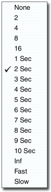Averaging options for real-time measurements in Smaart fall into four main types, arithmetic (FIFO), exponential (Fast and Slow), Infinite (Inf), and a proprietary hybrid technique we refer to simply as Variable. Variable averaging is specified by overall time constant (1 - 10 seconds).

FIFO Averaging (2, 4, 8, 16)

Beginning with the simplest case, FIFO averaging takes the "arithmetic" mean for each frequency data point over the most recent 2, 4, 8, or 16 FFT frames. For example if you want to average over the last 8 FFTs, then at each frequency you simply add up the last eight magnitude values measured for that frequency and divide by eight. The term FIFO (First-In, First-Out) refers to the fact that this is a moving average wherein the oldest value is retired from the average each time new data comes in. Another name for this type of average is a rectangular moving average or "boxcar" average, referring to the fact that every value in the average is given equal weight.

FIFO averaging works well when your measurement data is fairly stable and you want to integrate over a fairly short period of time. It may not be the best choice for system tuning in noisy environments as it offers relatively poor noise rejection compared to some alternatives, requires massive amounts of memory to achieve long time constants often required for acoustic measurement, and responds slowly to changes in EQ filter parameters and other settings when averaging over longer periods of time.

Exponential Averaging (Fast and Slow)

The Fast and Slow averaging options for real-time measurements are first-order exponential moving averages that mimic the characteristics of Fast and Slow time integration in standard sound level meters. These are handy options when you want to relate the frequency content of sound to overall sound pressure level (SPL). Exponential averaging differs from FIFO averaging in that it is a weighted average, wherein the oldest data is given relatively less weight than the newest. This type of average offers better responsiveness to changes than FIFO averaging but can take longer to stabilize and may yield poorer long-term stability than a FIFO average of similar length. Also the Slow setting has a time constant of just one second and when measuring in noisy environments we often want to integrate over several seconds.

Variable Averaging (1-10 Seconds)

Variable averaging in Smaart 7 utilizes a proprietary algorithm that seeks to combine the most desirable characteristics of FIFO and exponential moving averages. Smaart's variable averager stabilizes quickly and responds relatively quickly to EQ and other settings changes, while still providing better stability and immunity to transient events than FIFO averages of similar length. With variable averaging you select the desired length for your integration window in seconds and Smaart figures out how many individual measurements it needs to integrate to achieve it.

Infinite Averaging (Inf)

Infinite averaging a similar to FIFO averaging except that is a cumulative average where the oldest data is never removed. infinite averaging works well when you want to get the cleanest possible picture of the long-term response of the stable system. You can average over several minutes if you like, reducing noise and other transient events to negligible quantities. It is not such a great choice when you are actively making changes that affect the systems frequency response however, in that you have to keep flushing and restarting the average to see the effects of changes.

Polar vs. Complex Averaging (Transfer Function Only)

In addition to the options above that are common to all real-time frequency domain measurements, for transfer function measurements you can also select the type of data to be averaged for the magnitude display. In spectrum measurements complex data from the FFT is always translated into polar form (phase and magnitude) before averaging. In transfer function measurements, averaging for the phase displays always done using complex numbers (real and imaginary). The phase display would tend to regress to the zero line otherwise. For transfer function magnitude data, you have your choice of averaging polar or complex data – sometimes referred to as RMS and vector averaging. Magnitude averaging type (Mag Avg Type) is a global option for transfer function measurements and is set from the global options section in the Group Manager.

In general, complex (vector) averaging is considered by many to offer somewhat better noise rejection and to be a better predictor of subjective speech intelligibility than polar (RMS) averaging. Polar magnitude averaging tends to be somewhat more forgiving in circumstances where any sort of time variance is present in the system under test, due to such factors as wind, air currents or mechanical movement. Polar (RMS) is also considered by some to be the more musical of the two, perhaps owing to the fact that it tends to reject less reverberant energy as noise.